Can Light Travel Faster Than Light? At TRAVELS.EDU.VN, we delve into this fascinating question, exploring the boundaries of physics and engineering. Discover potential solutions and understand the challenges, all while planning your next adventure with unique travel experiences. Explore space demon concepts, wormhole travel potential, and engineering solutions that can solve the mysteries of the universe with TRAVELS.EDU.VN.
1. Building a Warp Drive: Is Faster-Than-Light Travel Possible?
Science fiction is full of ideas about traveling faster than light, but real physics has generally assumed that nothing can move through space faster than light. Is this really true? Our model for fundamental physics lets us analyze this question. While it’s complex, I suspect that exceeding the speed of light isn’t physically impossible, but an engineering challenge. Think of it as an irreducibly hard engineering problem, one that might not be solvable with the resources we have in our universe.
However, there might be a clever engineering solution, a way to “move through space” faster than light. To define “faster than light,” we must consider space tunnels like wormholes and the possibility of building them. Even if no tunnel exists, could we traverse space faster than light to get somewhere new?
Consider gas molecules bouncing around a room. A special molecule, perhaps a speck of dust or a virus particle, might know enough about the air molecules to avoid being buffeted, allowing it to travel much faster than diffusion. This requires knowledge and computation, but the limit on the molecule’s speed becomes an engineering question rather than a physical impossibility.
Similarly, space in our theory has a complex structure with parts acting in seemingly random ways. “Moving through space” faster than light becomes a question of whether a “space demon” can compute fast enough to “hack space”. It’s about exploring computational power, potential applications, and new avenues of research. At travels.edu.vn, we believe that even seemingly impossible ideas can lead to breakthroughs.
2. Understanding Space and Time: Our Model’s Framework
In standard physics, space is a background, a manifold with 3 coordinate values for every position. Our model sees space differently; it has definite, intrinsic structure, and everything in the universe is defined by it. Everything is “made of space.” We think of water as a continuous fluid, but it’s made of discrete molecules at a small scale. Space, I suspect, is similar. At a small enough scale, there are discrete “atoms of space,” making it appear continuous on a large scale.
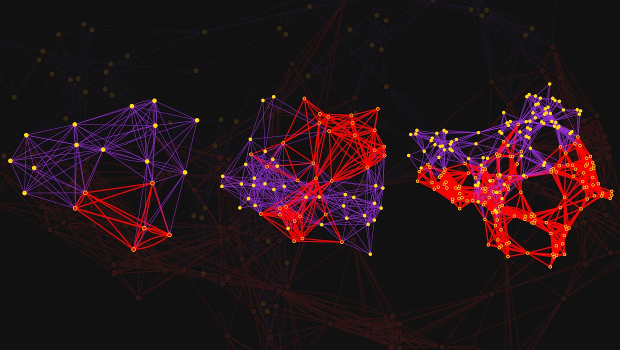
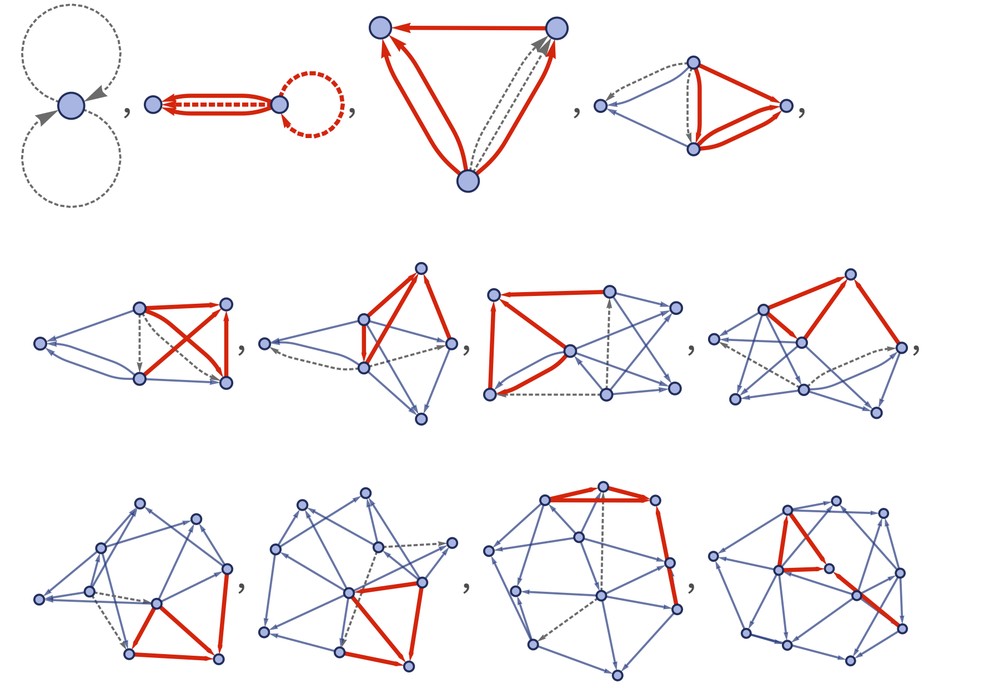
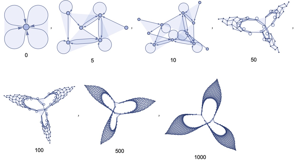
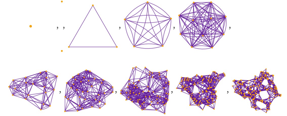
In our model, these “atoms of space” are abstract elements related to others. Mathematically, the structure is a hypergraph, where nodes (atoms of space) are connected by hyperedges. A small scale example might look like this:
 Graph3D
A slightly larger scale might be:
 Graph3D
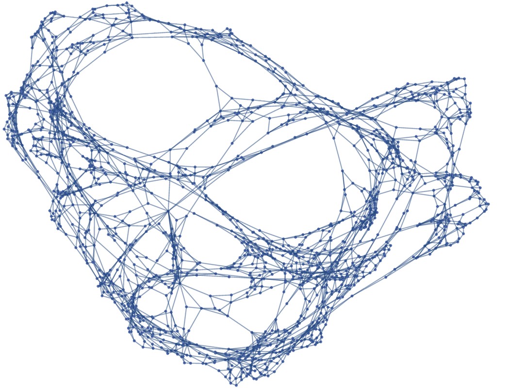
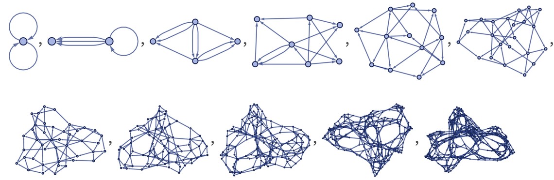
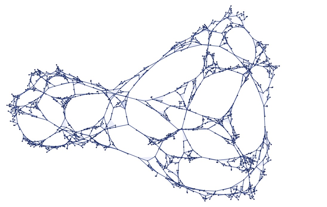
Our actual universe might have a hypergraph with around 10400 nodes. How does this giant hypergraph behave like continuous space? The nodes can be seen as forming a 2D grid on a curved surface:
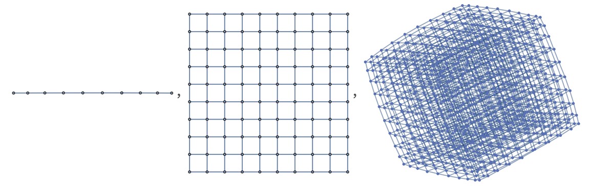
There’s nothing intrinsic that determines the effective dimensionality of space in our model. Here are several possible (hyper)graphs that behave like space in different dimensions:
 GridGraph
Introducing the “geodesic ball,” a region in the (hyper)graph reached by following at most r connections, is helpful. In a (hyper)graph that limits to d-dimensional space, the number of nodes in the geodesic ball grows like *rd. Curved space (like on a sphere’s surface) has a correction to rd* proportional to the curvature.
Just as fluid properties are derived from the large-scale aggregate dynamics of discrete molecules, space properties are derived from the large-scale aggregate dynamics of nodes in our hypergraphs. Excitingly, it seems we get exactly Einstein’s equations from general relativity. If space is a collection of elements in a “spatial hypergraph,” what is time? Unlike standard physics, it’s a reflection of the computation process by which the spatial hypergraph is updated.
3. Time as Computation: Causal Graphs and Reference Frames
Let’s say our underlying rule for updating the hypergraph is:
 RulePlot
A sequence of updates according to this rule might look like:
 EventsStatesPlotsList
Going further, we might get:
 StatesPlotsList
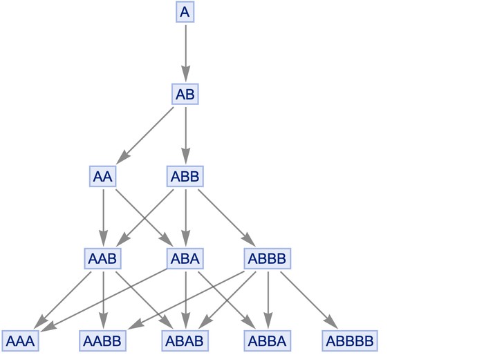
The underlying rule defines how a local piece of hypergraph should be updated. If several pieces have that form, it doesn’t specify which should be updated first. Once an update is done, it affects subsequent updates, creating a “causal graph” of causal relationships.
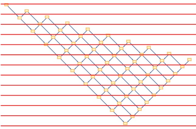
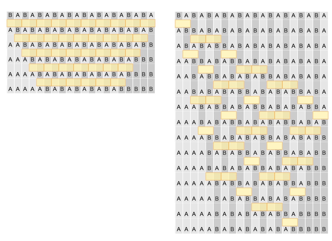
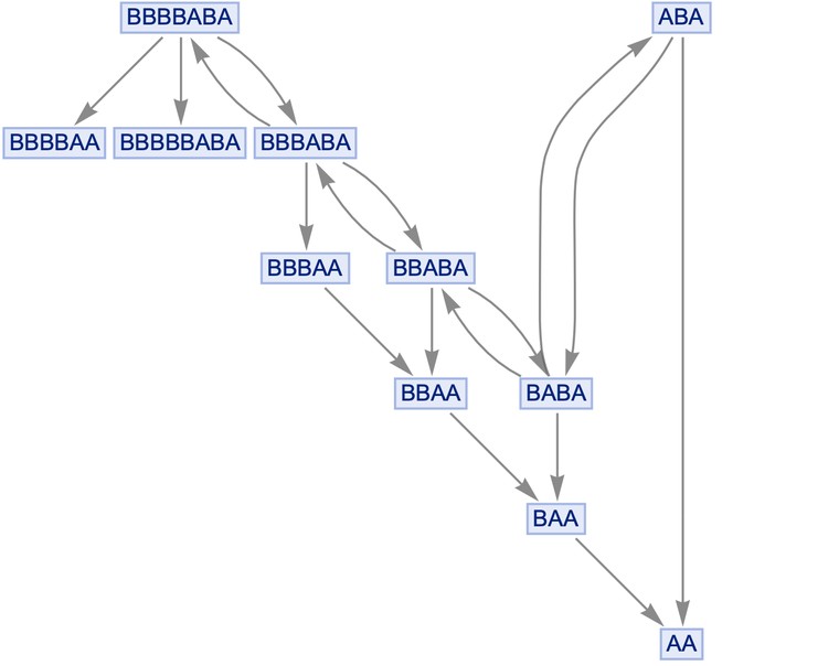
To see this more easily, consider strings of characters updated by the rule BA → AB:
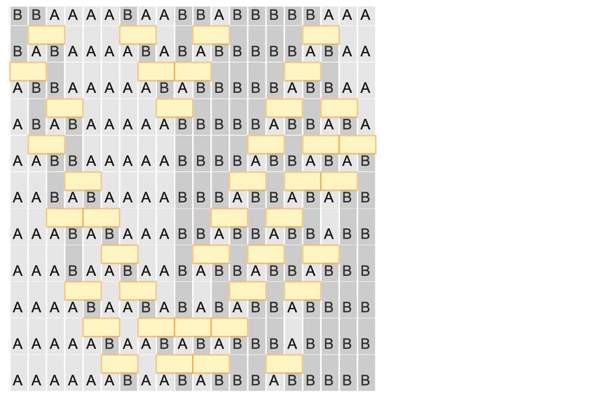 SubstitutionSystemCausalPlot
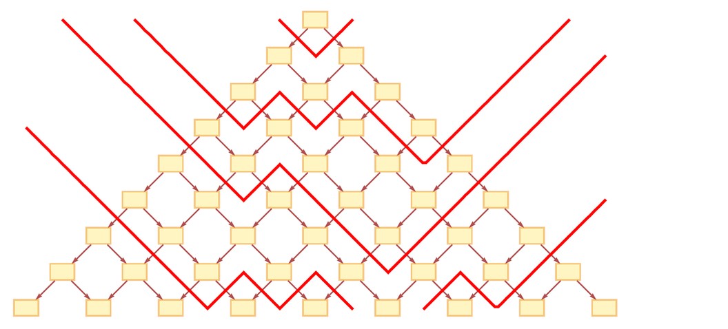
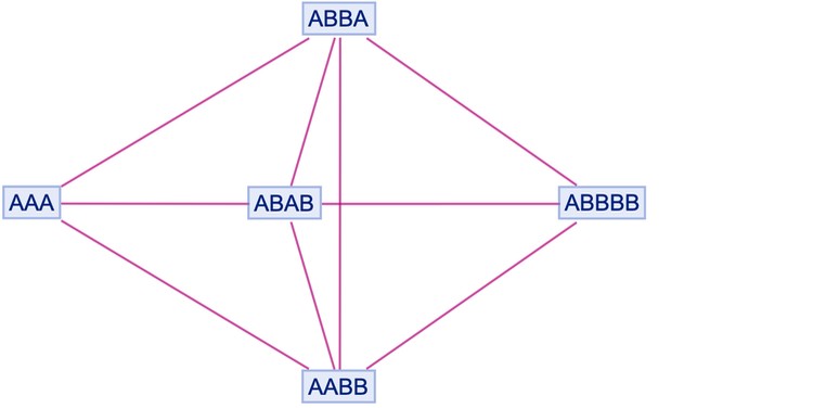
The yellow boxes indicate “updating events,” joined by a causal graph representing which event affects others:
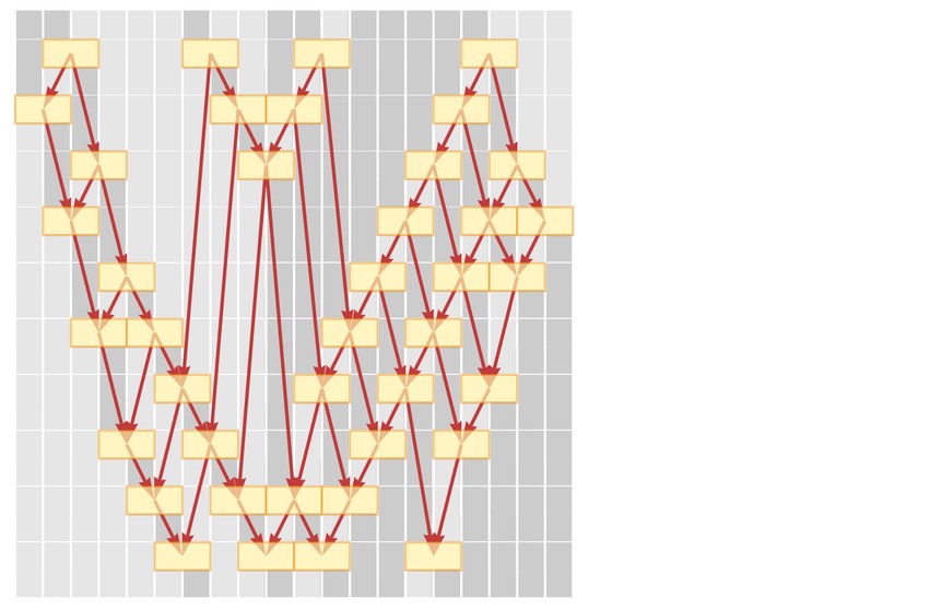 SubstitutionSystemCausalPlot
An observer inside the system only sees events and their causal connections. Describing what’s happening requires talking about events happening “at a certain time” and others later. We want to define “simultaneity surfaces” or a “reference frame.” Here are two choices:
The second one can be reinterpreted as:
 CausalGraphPlot
This corresponds to a reference frame with a different speed, like in special relativity. Our rule has the property of causal invariance—it doesn’t matter “at what time” an update is done; we always get the same causal graph. This is why we can derive special relativity even though space and time start differently in our models. Given a reference frame, we can “reconstruct” the system’s behavior from the causal graph. The system seeming to “take longer to do its thing” in the second reference frame reflects relativistic time dilation:
 GraphicsRow
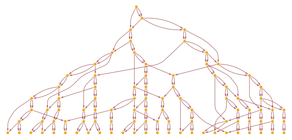
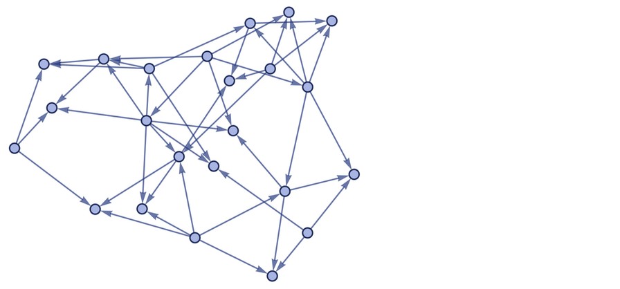
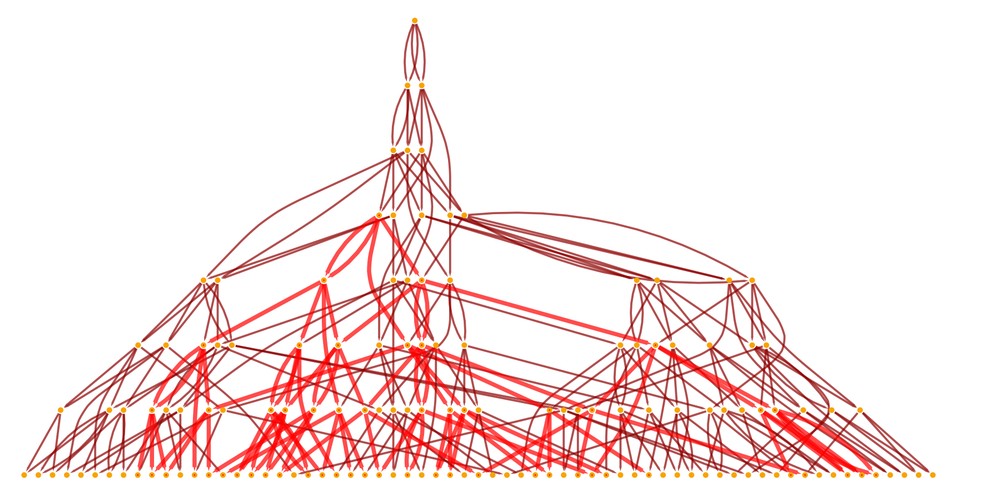
Like with strings, we can draw causal graphs for updating events in spatial hypergraphs. Here’s an example:
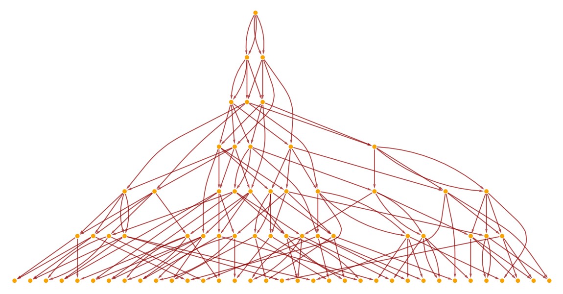 LayeredCausalGraph
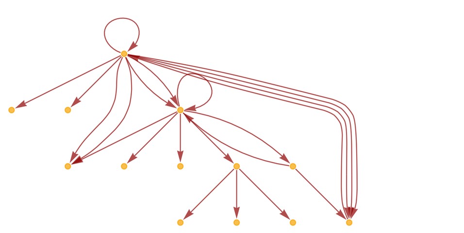
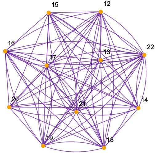
Again, we can set up reference frames to define “simultaneous” events. The only constraint is that no events in a slice can be timelike separated; they must be spacelike separated, defining a purely spacelike hypersurface. When drawing a causal graph, we pick relative orderings of possible updating events. Our models allow all possible orderings, constructing a whole multiway graph of possibilities. Here’s the multiway graph for the string system:
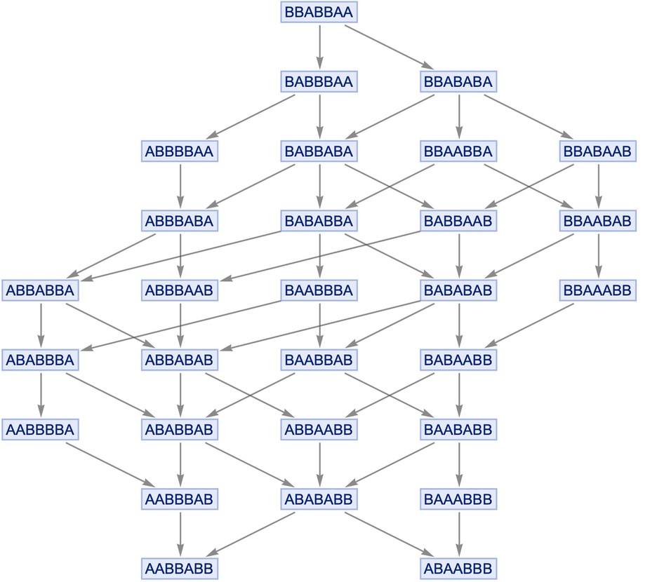 StatesGraph
Each node is a complete state, and a path through the system is a possible history with a corresponding causal graph.
4. Quantum Mechanics: Branchial Space and Entanglement
The fact that we get a multiway graph makes quantum mechanics inevitable in our models. Like reference frames help us understand space and time, “quantum observation frames” help us understand multiway graphs. The analog of space is “branchial space“: a space of quantum states, with connections defined by their relationship on branches.
Just as we define a spatial hypergraph for “points in space,” we define a branchial graph for relationships (entanglements) between quantum states in branchial space:
StatesGraph
We can derive the Einstein equations as a large-scale limiting description of spatial hypergraphs. Similarly, we can find the large-scale limiting behavior for multiway systems, which seems to give us the Feynman path integral for quantum mechanics! Motion in branchial space is also possible, and we have a maximal entanglement rate ζ that limits how fast we can explore different quantum states. Just as we ask about “faster than c,” we can talk about “faster than ζ.”
5. Space Tunnels: Bypassing the Conventional
Traditional general relativity sees space as a continuous manifold. Our models describe what space is made of, implying new and different phenomena. Imagine a hypergraph as a simple 2D grid:
 GridGraph
In the limit, this is like 2D Euclidean space. Now, add some “long-range threads”:
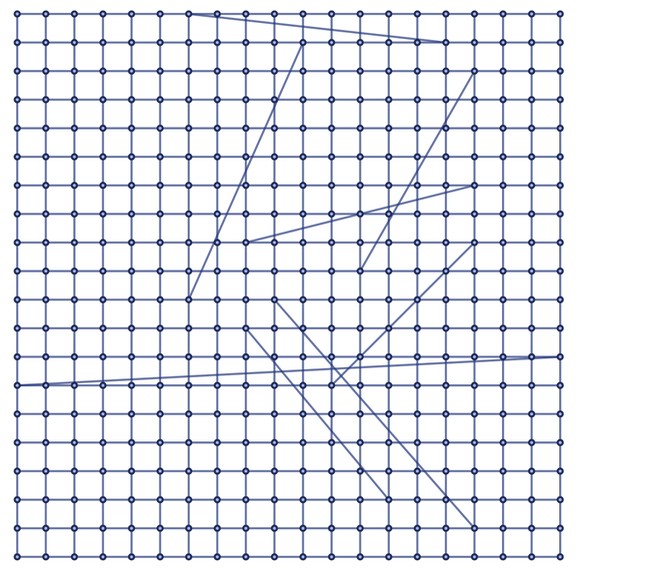 EdgeAdd
Here’s a different rendering of the same graph:
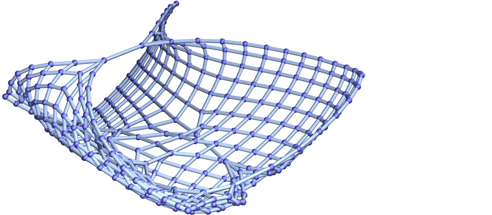 Graph3D
Some nodes will have distances like in ordinary 2D space, but some will be “anomalously close” due to shortcuts along the long-range threads. If we move around the graph, traversing a single connection per time interval, our view of “what space is like” is based on the general graph structure (ignoring the long-range threads). We conclude how far we can go in a time and the maximum speed to “go through space”. But what if we encounter one of the long-range threads? We get from one “place in space” to another much faster than our deduced maximum speed.
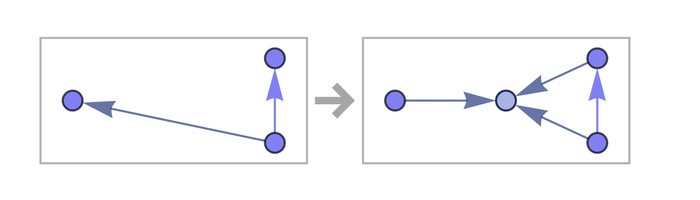
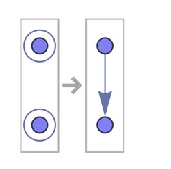
There are many ways to create “long-range threads,” defining “space tunnels” to evade usual speed-of-light constraints. These can be persistent or transient. But what happens when something “goes through it”? How does a tunnel form? Space tunnels are a general concept, but wormholes are a special case in general relativity. General relativity describes space as a continuum where you can’t have “just a few long-range threads.” The best you can do is imagine a “handle in space,” providing an alternative path:
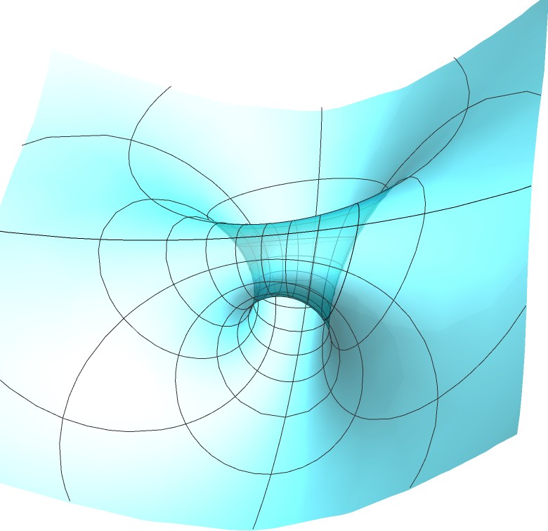 Wormhole diagram
How would such a non-simply-connected manifold form? Maybe like gastrulation in embryonic development. Mathematically, you can’t continuously change the topology of something continuous; there has to be a singularity. This has been tricky in general relativity. In our models, there’s not the same constraint because you don’t have to “rearrange a whole continuum”; you can “grow a handle one thread at a time”.
Here’s an example of this happening with a rule that “knits handles,” providing “shortcuts” between “separated” points in patches of 2D Euclidean space:
 Labeled
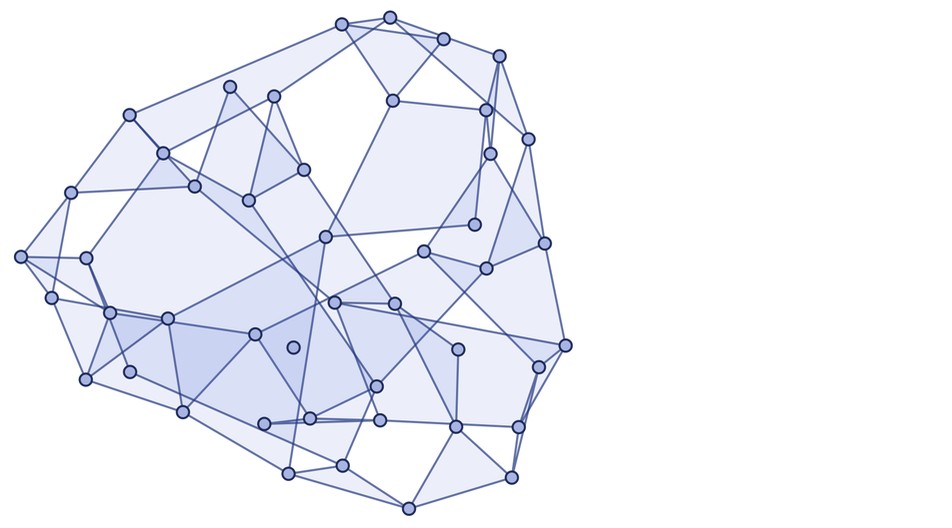
In our models, space can have exotic forms without continuity constraints. Dimension isn’t limited to integers; it’s defined by asymptotic growth rates of balls and can have any value. Here’s a case approximating 2.3-dimensional space:
 FinalStatePlot
Although distance and other geometric concepts can be defined on such a graph, you can’t assign nodes to positions with coordinates, as in integer-dimensional space. With a manifold, you pick a dimension and stick to it. In our models, dimension becomes a dynamical variable that can change with position and time. A “space tunnel” can be a region of space with higher or lower dimension. Lower-dimensional tunnels connect specific sets of “distant” points, while higher-dimensional ones are “switching stations” that bring points on their boundaries closer.
6. Negative Mass and Wormholes: Exotic Phenomena and Their Challenges
If we somehow get a space tunnel, what happens to it? General relativity suggests it’s hard to maintain a wormhole. A wormhole is defined by geodesic paths converging upon entry and diverging upon exit. In general relativity, mass makes geodesics converge, but gravitational repulsion is needed to make them diverge. This requires negative mass.
Normally, mass is positive. However, dark energy has to have negative mass, and there are mechanisms in traditional physics that lead to negative mass, revolving around where one sets zero. Normally, we set “the vacuum” to have zero energy (and mass). But even in traditional physics, the vacuum has a constant intensity of the Higgs field and vacuum fluctuations. If these exist everywhere, we can set our zero of energy to include them. If something reduces their effects, we see negative mass. The Casimir effect is one example.
Imagine vacuum inside a box. The box cuts out some vacuum fluctuations, leading to negative energy density inside the box. This is observable with metal boxes, but its effects in spacetime or gravitational settings aren’t clear. (In 1981, I wrote two papers about the Casimir effect with Jan Ambjørn, but we never wrote the planned “…: 3. Gravitational” paper. I’m now curious what the results would have been. Our paper #1 computed Casimir effects for boxes of different shapes, implying that changing shapes in a cycle could “mine” energy from the vacuum. This was later suggested as a method for interstellar propulsion, but requires an infinitely impermeable box, perhaps using gravitational effects and event horizons…)
Traditional physics has conflicted quantum field theory’s vacuum (infinite energy density) with general relativity’s vacuum (zero energy density). In our models, the vacuum has even more structure. Space isn’t separate; it’s a consequence of the spatial hypergraph’s structure. Matter, particles, and quantum fields are features of this hypergraph. Vacuum fluctuations are part of space’s formation.
Our hypergraph isn’t static, knitted together by update events. The energy of a region relates to the updating activity there (or the flux of causal edges through spacelike hypersurfaces). So, if there’s a region of less activity, it has negative energy relative to the “normal vacuum.” Whatever reduces activity could be called a “vacuum cleaner.” We don’t know if they exist, but they lead to wormholes being maintained (because geodesics diverge where a vacuum cleaner has operated).
While a wormhole requires negative mass and vacuum cleaners, other space tunnel structures might not. They operate outside general relativity, so its singularity theorems don’t apply. Instead, they must be analyzed directly in our models. Why not simulate a space tunnel configuration to see what happens? Computational irreducibility is the problem. A simulation might show stability for a billion steps, but that’s far from human-level timescales. There may be no way to determine the outcome for a given number of steps except by doing that irreducible amount of computational work.
Even if we “engineer” a space tunnel, there’s no systematic way to guarantee it’ll “stay up”; it might require an infinite sequence of “tweaks.” Before that, we must figure out how to construct one in the first place.
7. The Absence of Time Travel: Maintaining Causal Order
In general relativity, a wormhole connects different places in spacetime, allowing shortcuts between different parts of space and time, potentially allowing time travel. A causal connection from the future to the past isn’t strange in a perfectly periodic system, but it’s a future determined by the periodic behavior.
It’s complicated to see how this works mathematically in general relativity, but the presence of wormholes presumably limits consistent solutions to ones where past and future are locked with something like periodic behavior. In traditional physics, “time is just a coordinate,” so there’s “motion in time” like we have in space. In our models, space and time are different. Space is the structure of the spatial hypergraph, and time is the computational process of applying updates, showing computational irreducibility.
So while we go backwards and forwards in space, the progress of time is associated with the progressive performance of irreducible computation by the universe. One can compute what will happen (or has happened), but only by following the actual steps. In our models, the causality of events is tracked, represented by the causal graph. Each connection is the smallest unit of progression in time.
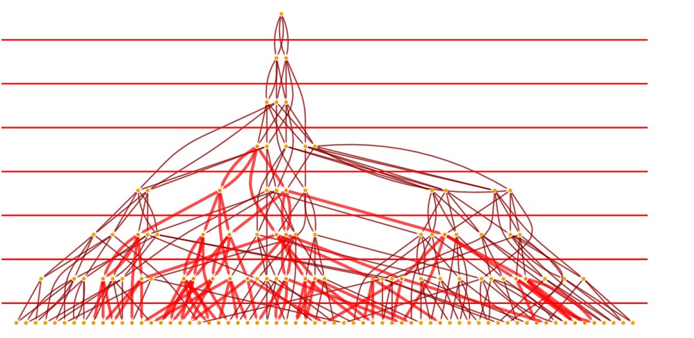
Let’s look at a causal graph again:
 LayeredCausalGraph
It contains no cycles. There’s a definite “flow of causality.” There’s a partial ordering of what events can affect, and there’s never looping back. There are different ways to define “simultaneity surfaces”:
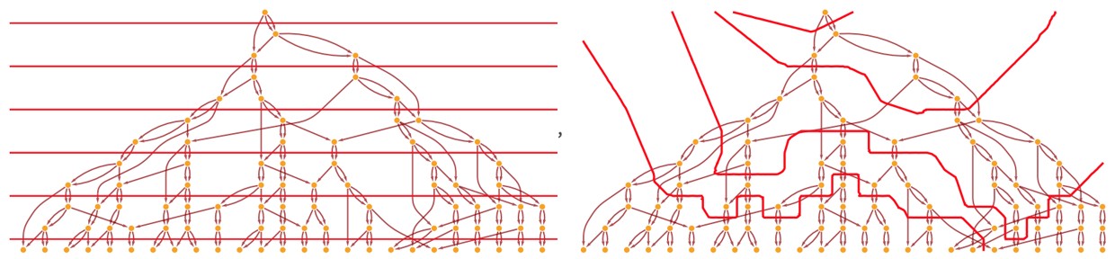 Show
Show
There’s always a way to do it so that events in a slice are “causally before” events in subsequent slices. Whenever the underlying rule has causal invariance, things have to work this way. If we break causal invariance, other things can happen. Here’s a multiway system for a (string) rule that doesn’t have causal invariance, where the same state can repeatedly be visited:
 Graph
Graph
The corresponding (multiway) causal graph contains a loop:
 LayeredGraphPlot
This loop represents a closed timelike curve, where the future can affect the past. We can’t construct a foliation in which “time systematically moves forward.” But the presence of these loops is different from space tunnels. A space tunnel is spatial hypergraph connectivity that makes the distance between two points shorter than expected from the hypergraph’s structure, connecting different places in space. An event at one end can affect distant events, but those events must be “subsequent events” with respect to the partial ordering defined by the causal graph.
“Jumping” between distant places in space doesn’t require “traveling backwards in time.” Even as effects propagate through space tunnels faster than light, time can still progress to places that seem distant.
8. Causal Cones and Light Cones: Differentiating Effects and Their Boundaries
Now, let’s discuss faster-than-light effects in our models. When an event occurs, it can affect a cone of subsequent events in the causal graph. When the causal graph is a simple grid, it’s straightforward:
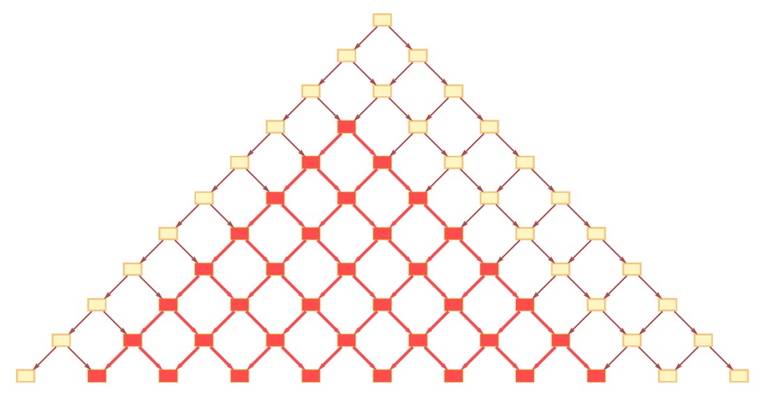 HighlightGraph
But in a more realistic causal graph, it’s more complicated:
 HighlightGraph
The “causal cone” of affected events is well-defined. How does this relate to space and time? We typically think of light cones. Given a light source, where in space and time can it affect?
The causal cone isn’t exactly the light cone. The light cone is defined by positions in space and time, making sense if we have a manifold representing continuous spacetime, where we can set up coordinates. But in our models, there’s not intrinsically anything like that. We can say what element in a hypergraph is affected after some events, but there’s no a priori way to say where that element is in space. That’s only defined in some limit, relative to the whole hypergraph.
This is the nub of the issue: causal relationships are immediately well-defined, but spatial ones aren’t. One event can affect another through a single connection in the causal graph, but those events might be at different ends of a space tunnel that traverses a large distance. There are related issues centering around what space really is. Can we define an instantaneous snapshot of space? That’s what our reference frames, foliations, and simultaneity surfaces are about. They specify which collection of events happened when we “sample space’s structure.” There’s arbitrariness to this choice, like in relativity’s reference frames.
Can we choose any collection of events consistent with the partial ordering defined by the causal graph? Let’s imagine a weird foliation:
 Show
Show
The spatial hypergraph could be very different. But for now, let’s ignore this and pick a “reasonable” foliation. Then, what’s the “projection” of the causal cone onto the instantaneous structure of space? What elements in space are affected by an event?
Let’s look at an example with the “flat” foliation:
 HighlightGraph
Here are spatial hypergraphs associated with successive slices, with the parts contained in the causal cone highlighted:
 Images
For the first 3 slices, the event hasn’t happened yet. After that, we see the event’s effect spreading across successive spatial hypergraphs, the light cone expanding with time. The critical question is: how fast does the light cone expand? How much space does it traverse per time unit? What’s the effective speed of light here? It’s clear from the pictures that this is a subtle question.
The speed of light is measured in units like meters per second. We can get a speed in spatial hypergraph edges per causal edge. Each causal edge corresponds to an elementary time elapsing. Quoting elementary time in seconds (say 100–100 s) defines the second. Similarly, each spatial hypergraph edge is a distance of an elementary length. If in t elementary times, the light cone advances by α t spatial hypergraph edges, or α t elementary lengths, what is α t in meters? It has to be α c t, where c is the speed of light, defining the speed of light.
It’s at some level a tautology to say the light cone advances at the speed of light. But it’s more complicated. In continuum space, it’s consistent to say the speed of light is the same in every direction. When we project our causal cone, we can’t really say that anymore. To know what happens, we have to characterize space more. In our models, causal effects are clear, but where these effects show up in what we call space is far from clear.
9. Distance Measurement: Proxies for Physical Space
Speeds are complicated because positions and times are hard to define. Consider cellular automata, where we set up a grid in space and time. How fast can an effect propagate? If we change one cell, by how many cells per step can the effect expand? Here are some results:
The speed of expansion can vary, but the absolute maximum is 1 cell/step. This is straightforward to understand from the underlying rules:
 RulePlot
The rule “reaches” one cell away, so 1 cell/step is the maximum rate. Something analogous happens in our models. Consider a rule like:
 RulePlot
The rule only “reaches” a limited number of connections away. In each updating event, only elements within a certain range can “have an effect” on each other. But this is only a local statement. While the rule implies effects can only spread a certain distance in an update, it doesn’t say the “relative geometry” of successive updates or what might be connected to what. Unlike in a cellular automaton, there’s no immediate global consequence to the rules being local with respect to the hypergraph.
The rules don’t strictly have to be local. If the left-hand side is disconnected, as in:
 RulePlot
then an update can pick up elements from anywhere, even disconnected parts. Anything anywhere can immediately affect anything else. But with this rule, there doesn’t seem to be a way to build up anything with the locality properties of what we think of as space. Given a spatial hypergraph, how do we figure out “how far” it is from one node to another?
It’s easy to find the graph distance: the geodesic path from one node to another, counting connections. But this is an abstract distance. How does it relate to what we measure “physically”? We have a hypergraph representing everything, and we want something—itself part of the hypergraph—to measure a distance in the hypergraph. In traditional relativity, we measure distances by looking at arrival times of light signals or photons, assuming an underlying space structure. In our models, photons have to be part of the spatial hypergraph; they’re “pieces of space.”
When we study the spatial hypergraph directly, we’re operating far below the level of photons. To compare what we see with actual distance measurements, we need a proxy for physical distance that we can compute directly on the spatial hypergraph.
A simple possibility is just graph distance, ignoring the directedness of hyperedges. In large hypergraphs, this shouldn’t make much difference. Another good proxy is derived from the causal graph. It’s the analog of beacons signaling each other over time. We can say it’s the analog of a branchial distance for the causal graph.
Construct a causal graph:
 LayeredCausalGraph
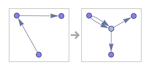
Look at the events in the last slice. For each pair, look at their ancestry. If they have a common ancestor on the step before, connect them. The result is the graph:
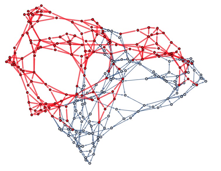
 SpatialReconstruction
This is a “reconstruction of space,” based on the causal graph. In the appropriate limit, it should be essentially the same as the original hypergraph:
 FinalStatePlot
It’s important to understand the differences between these graphs. In the spatial hypergraph, nodes are fundamental elements, and hyperedges are relations. In the causal graph, nodes are updating events, joined by edges that are causal relationships. The “spatial reconstruction graph” has events as its nodes, with edges representing immediate common ancestry. When an event “causes” other events, it’s like “starting an elementary light cone” that contains the others. The causal graph “knits together” the light cones. The spatial reconstruction graph uses the fact that two events lie in the same light cone to infer that they’re “close together.”
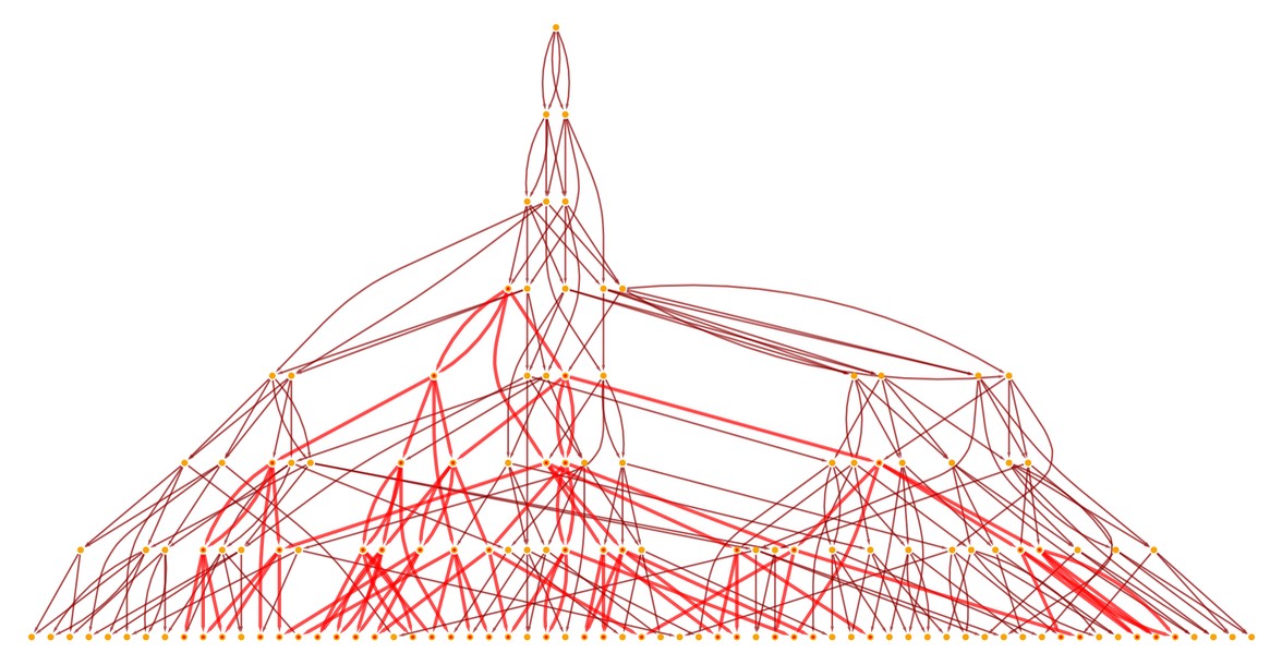
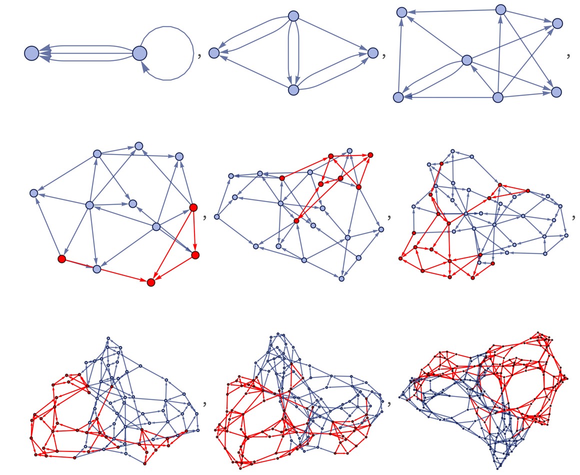
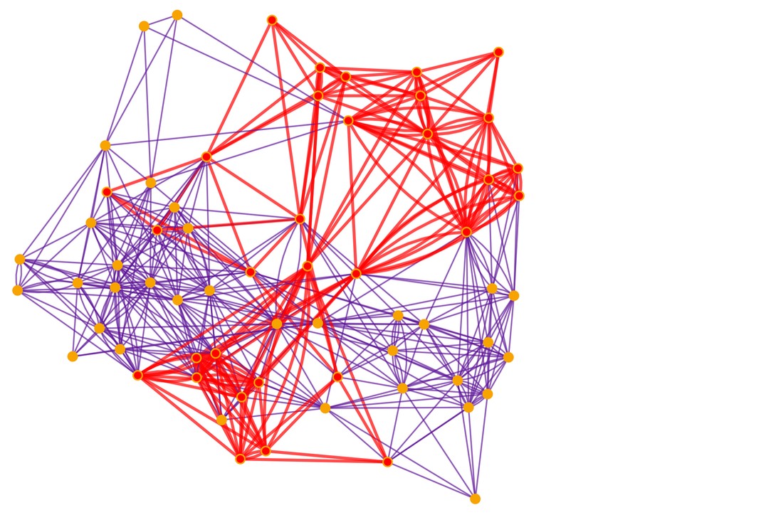
There’s an analogy to quantum mechanics. We start from multiway graphs of quantum states, take slices, and construct branchial graphs, joining states that have an immediate common ancestor. In the branchial graph, we join states in the same “entanglement cone.” The resulting branchial graph is a map of a space of quantum states and their entanglements:
 MultiwaySystem
The spatial reconstruction graph is the same idea: a branchial graph, but from the causal graph. (The spatial reconstruction graph is a new graph, edges colored with a blend of our “branchial pink” and spatial hypergraph’s blue-gray.) In the spatial reconstruction graph, we join events when they have a common ancestor one step before.
We can generalize this, allowing common ancestors more than one step back. Going even two steps back causes almost all events to have common ancestors:
 SpatialReconstruction
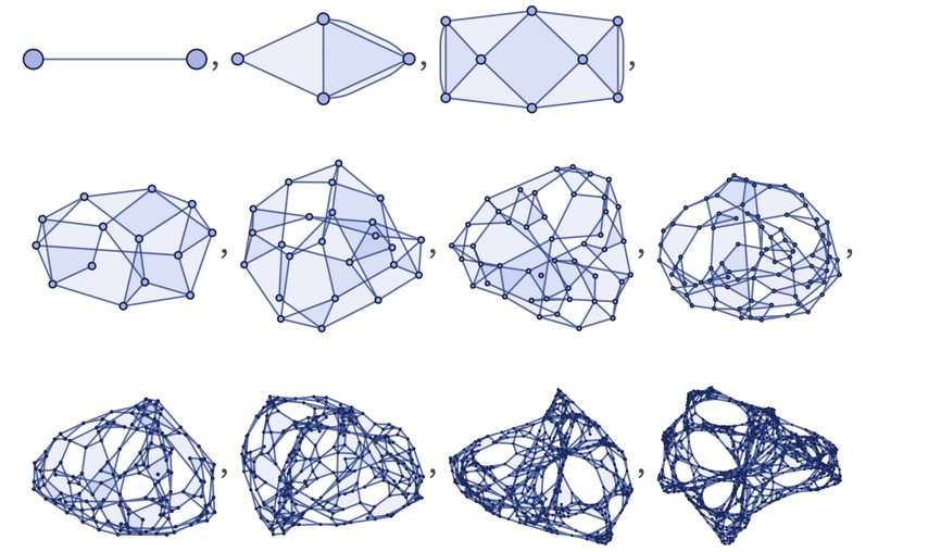
If we go enough steps back, every event shares a common ancestor: the “big bang” event. Let’s say we have a rule that leads to spatial hypergraphs:
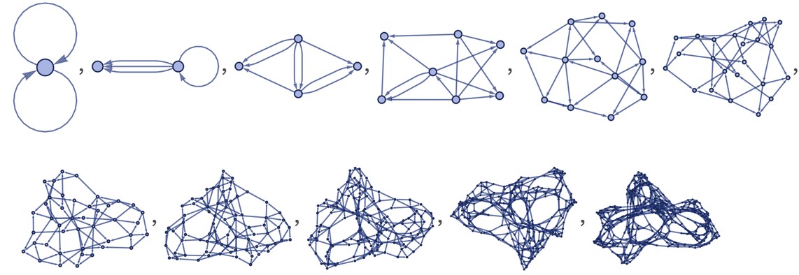 StatesPlotsList
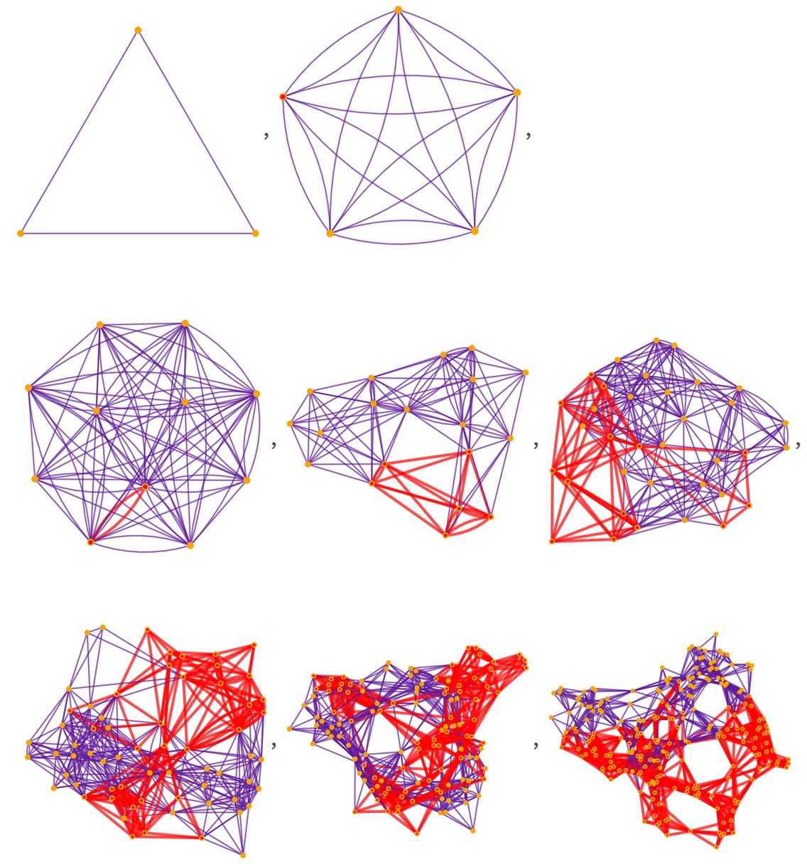
We can compare these with the spatial reconstruction graphs from the causal graph for this system. Here are the results on successive steps, allowing a “lookback” of 2 steps:
 Table
Table
As the number of steps increases, there’s increasing commonality between the spatial hypergraph and the spatial reconstruction graph. The spatial reconstruction graphs we’ve drawn aren’t the only ways to get a proxy for physical distances. We can look at common successors, rather than common ancestors.
Another change is to look not at a spatial hypergraph where the nodes are elements and the hyperedges are relations, but at a “dual spatial hypergraph” where nodes are relations and hyperedges are associated with elements, recording which relations share a given element. For the spatial hypergraph:
 FinalStatePlot
the corresponding dual spatial hypergraph is:
 UnorderedHypergraphPlot
and the sequence of dual spatial hypergraphs corresponding to the evolution above is:
 Table
Table
There are other possibilities, particularly if one goes “below” the causal graph, looking at causal relations between specific relations in the spatial hypergraph. The main takeaway is that there are various proxies we can use for physical distance. In the limit of a large system, all should give compatible results. In small graphs, they won’t quite agree, so we may not be sure what to say the distance between two things is.
10. Causal Balls vs. Geodesic Balls: Measuring and Interpreting Speed
To measure speed, we divide distance by elapsed time. When constructing space and time, it’s not straightforward to say what we mean by distance and elapsed time. As a first approximation, let’s ask about the effect of a single event. The effect is captured by a causal cone:
 HighlightGraph
The elapsed time associated with a particular slice is the graph distance from the event at the top of the cone to events in the slice. So now we see how far the event spreads in space. The first step is to “project” the causal cone onto instantaneous space. We can do this with the spatial hypergraph:
 HighlightEffectiveSpatialBallPlot
To align with “elapsed time,” it’s better to use the spatial reconstruction graph, whose nodes are events:
 HighlightGraph
Let’s “watch the intersection grow” from slices of the causal cone, projected onto spatial reconstruction graphs:
 Table
Table
How “wide” is that area of intersection? The pictures make it clear it’s not trivial to answer. In the continuum